
For one of my applications it is necessary to know the geopotential at each model level of the ERA5 data. Since ERA5 and ERAI only store the geopotential at the surface, it may not be immediately obvious how to arrive at the remaining values. This post deals with how to achieve this. While shown for ERA5, the procedure is similar for ERA-Interim.
Model levels in ERA5
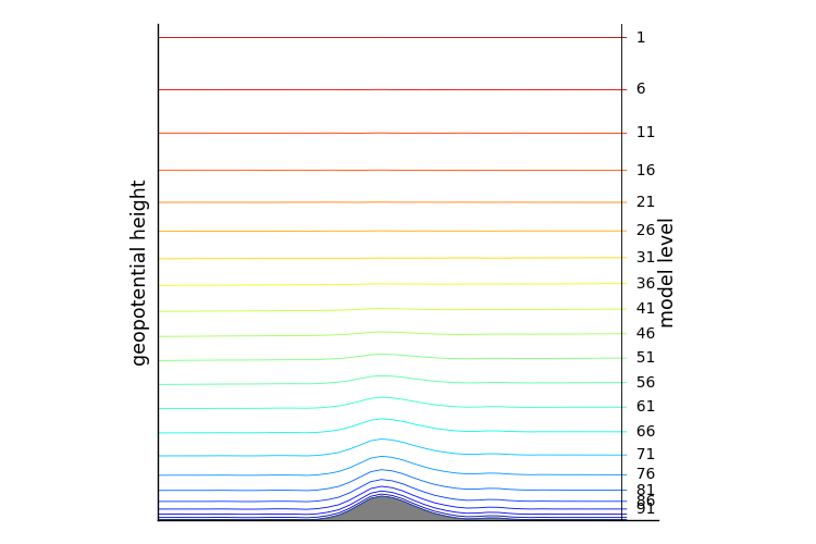
Essentially the vertical coordinate system in ERA5 is chosen as such that closer to the surface the model levels follow the topography while farther up they follow pressure levels with a transitional region in between. Some of the details of this are summarized nicely here (for ERA-Interim). In ERA5 the levels are numbered from top to bottom, with 1 being the topmost layer and 137 the one closest to the surface. This is illustrated by the following plot:
The levels shown above are actually referred to as full model levels. Each of these full model levels is defined and bounded by a half-level above and a half-level below. Note that the full model levels are associated with a volume while the half-levels correspond to an area – the interface between two full model levels.
Calculating pressure at half model levels
While not necessary right now we’ll need information about the pressure at the half-levels (interfaces between full model levels) later on. The equation that defines the pressure at each half-level is
![\[ p_{k+1/2} = a_{k+1/2} + b_{k+1/2}\,p_s \]](/wp-content/ql-cache/quicklatex.com-068eecc955dc4ae873a3adb90d013b6b_l3.png "Rendered by QuickLaTeX.com")
where  denotes the pressure at half-level
  ,
,  the surface pressure and
  and
and  constants that define the vertical coordinate.
Where do we get the values of the constants and from? Luckily the ECMWF lists them all in a nice table, complete with some exemplary values of quantities at half levels (pressure) and full-levels (pressure, geopotential altitude, geometric altitude, temperature and density).
Where is the half-level located? An easy way to think of this is to remember that levels are numbered from top to bottom. E.g. the smaller the value the higher up the associated model level will be. Adding k+1/2 then is the half-level below full model level k while k-1/2 is the half-level above.
The pressure at a full model-level k is given by the average of the pressure between the two bounding half-levels:
![\[p_k = \frac{1}{2}(p_{k-1/2} + p_{k+1/2})\]](/wp-content/ql-cache/quicklatex.com-2d10aee64178dc99f017736352f49017_l3.png "Rendered by QuickLaTeX.com")
The vertical discretisation and the remaining equations we need are documented in Part 3 of the IFS documentation (IFS 2015).
Geopotential at full model levels
The starting point is equation (2.22):
![\[ \phi_k = \phi_{k+1/2} + \alpha_k R_{\text{dry}}(T_v)_k \]](/wp-content/ql-cache/quicklatex.com-f49a1eb305c09fa835d44d13e3ef11c6_l3.png "Rendered by QuickLaTeX.com")
Here  is the geopotential at half-level ,
  the gas constant for dry air and
  the virtual temperature at full-level
  . The coefficient
  is defined as
  and for
  as
as
![\[ \alpha_k = 1-\frac{p_{k-1/2}}{\Delta p_k}\ln{\left(\frac{p_{k+1/2}}{p_{k-1/2}}\right)} \]](/wp-content/ql-cache/quicklatex.com-94598b542dd73db38015fde3fbea2c6d_l3.png "Rendered by QuickLaTeX.com")
To calculate  directly from fields available in ERA5 the following equation is applicable:
![\[ T_v = T \left\{ 1 + \left[ (R_{\text{vap}}/R_{\text{dry}} ) - 1 \right] q \right\} \]](/wp-content/ql-cache/quicklatex.com-19672dbf694fd6d596c04a09121e731f_l3.png "Rendered by QuickLaTeX.com")
Here  is the temperature,
  the specific humidity and
  the gas constant for water vapour.
This leaves us with as the only remaining quantity. It is given by equation 2.21 in IFS (2015):
![\[ \phi_{k+1/2} = \phi_S + \sum_{j=k+1}^N R_\text{dry} (T_v)_j \ln{\left( \frac{p_{j+1/2}}{p_{j-1/2}}\right)} \]](/wp-content/ql-cache/quicklatex.com-fd11155c3dece01e155e9a7473bdffd9_l3.png "Rendered by QuickLaTeX.com")
with  as the geopotential at the surface and
  as the number of full model-levels, which is
  in case of ERA5.
ERA5 data required
To actually carry out the calculation, the following ERA5 fields are required (parameter number in brackets)
- geopotential at the surface (129.128)
- pressure at the surface (134.128)
- temperature (130.128)
- specific humidity (133.128)
Here’s an example netcdf file that contains exactly this data for a region encompassing the South Island of New Zealand over two days (only model levels 30-137), plus a .csv file that contains the model-level defining constants  and
and  .
.
Python code example
The following code calculates the geopotential of a given ERA5 model level based on the data above. To run it you’ll need to download this library of mine from github [geopotcalc on github] and place it in a folder named ‘lib’ within the directory you’ll be running the following code from. Furthermore the python packages xarray, numpy and pandas should also be installed.
import lib.gpcalc as gpc
import xarray as xa
import pandas as pd

era5_ds = xa.open_dataset('./era5_ml_example.nc')
mldf    = pd.read_csv('./akbk.csv',index_col='n')

gpc.set_data(era5_ds, mldf, 137)
gpc.get_phi(130)  # calculates the geopotential at model level 130.
The output should look like this:
<xarray.DataArray (time: 48, latitude: 37, longitude: 45)>
array([[[ 2061.799 ,  2068.4844, ...,  9074.937 ,  9794.214 ],
        [ 2068.3455,  2071.648 , ..., 12285.38  , 12331.378 ],
        ...,
        [ 2031.0612,  2031.0513, ...,  2022.7593,  2029.4838],
        [ 2029.6093,  2035.5366, ...,  2021.2681,  2032.0813]],

       [[ 2062.8289,  2070.104 , ...,  9076.426 ,  9794.513 ],
        [ 2068.5178,  2072.9602, ..., 12283.5   , 12330.7705],
        ...,
        [ 2028.933 ,  2029.8497, ...,  2023.5824,  2032.0865],
        [ 2025.4272,  2032.5043, ...,  2023.407 ,  2032.3804]],

       ...,

       [[ 2045.6422,  2051.2817, ...,  9068.013 ,  9790.583 ],
        [ 2053.2986,  2057.6807, ..., 12275.755 , 12324.499 ],
        ...,
        [ 1981.8191,  1980.5361, ...,  1987.5459,  1996.2969],
        [ 1977.6063,  1985.1229, ...,  1987.896 ,  1998.8293]],

       [[ 2047.196 ,  2053.632 , ...,  9075.75  ,  9798.725 ],
        [ 2052.647 ,  2056.1565, ..., 12282.7   , 12331.903 ],
        ...,
        [ 1985.239 ,  1981.6675, ...,  1986.0985,  1996.3464],
        [ 1978.8458,  1985.9766, ...,  1985.4244,  1997.1885]]], dtype=float32)
Coordinates:
  * longitude  (longitude) float32 165.0 165.25 165.5 165.75 166.0 166.25 ...
  * latitude   (latitude) float32 -39.0 -39.25 -39.5 -39.75 -40.0 -40.25 ...
    level      int32 130
  * time       (time) datetime64[ns] 2015-02-01 2015-02-01T01:00:00 ...
So that’s essentially it. Most of it is already documented in IFS (2015), however, I found that actually finding this information was the hardest part. If there’s any errors or any questions arise from the above – don’t hesitate to contact me.
References
ECMWF, IFS. “Documentation–Cy40r1.” Part III: Dynamics and numerical procedures, ECMWF (2015). [link]